GSSTDA: Gene Structure Survival using Topological Data Analysis

Installation

You can install the development version from GitHub with:

library(devtools)
devtools::install_github("jokergoo/ComplexHeatmap")

devtools::install_github("MiriamEsteve/G-SS-TDA")
library(GSSTDA)

Loading data

The full data is the expression matrix,
the survival_time is a vector with time between disease diagnosis and death, or other type of event, (if there has been no death, until the end of follow-up),
the survival_event is a vector with information on whether or not the patient has died (or other type of event)
and the case_tag with information from each patient on whether he/she is healthy or not.

See GSSTDA documentation for further information.

data("full_data")
data("survival_time")
data("survival_event")
data("case_tag")

Declare the necessary parameters of the GSSTDA object.

The gen_select_type parameter is used to choose the option on how to select the genes to be used in the mapper. Choose between “Abs” and “Top_Bot”. The percent_gen_select parameter is the percentage of genes to be selected to be used in mapper.

# Gene selection information
gen_select_type <- "Top_Bot"
percent_gen_select <- 10 # Percentage of genes to be selected

For the mapper, it is necessary to know the number of intervals into which the values of the filter functions will be divided and the overlap between them (). Default are 5 and 40 respectively. It is also necessary to choose the type of distance to be used for clustering within each interval (choose between correlation (“cor”), default, and euclidean (“euclidean”)) and the clustering type (choose between “hierarchical”, default, and “PAM” (“partition around medoids”) options).

For hierarchical clustering only, you will be asked by the console to choose the mode in which the number of clusters will be chosen (choose between “silhouette”, default, and “standard”). If the mode is “standard” you can indicate the number of bins to generate the histogram (, by default 10). If the clustering method is “PAM”, the default method will be “silhouette”. Also, if the clustering type is hierarchical you can choose the type of linkage criteria ( choose between “single”, “complete” and “average”).

#Mapper information
num_intervals <- 5
percent_overlap <- 40
distance_type <- "cor"
clustering_type <- "hierarchical"
linkage_type <- "single" # only necessary if the type of clustering is hierarchical 
# num_bins_when_clustering <- 10 # only necessary if the type of clustering is hierarchical 
                                 # and the optimal_clustering_mode is "standard"
                                 # (this is not the case)

The package allows the various steps required for GSSTDA to be performed separately or together in one function.

OPTION #1 (the three blocks of the G-SS-TDA process are in separate function):

First step of the process: DGSA.

This analysis, developed by Nicolau et al. is independent of the rest of the process and can be used with the data for further analysis other than mapper. It allows the calculation of the “disease component” which consists of, through linear models, eliminating the part of the data that is considered normal or healthy and keeping only the component that is due to the disease.

DGSA_object <- DGSA(full_data, survival_time, survival_event, case_tag)

Second step of the process: Select the genes within the DGSA object created in the previous step and calcute the values of the filtering functions.

After performing a survival analysis of each gene, this function selects the genes to be used in the mapper according to both their variability within the database and their relationship with survival. Subsequently, with the genes selected, the values of the filtering functions are calculated for each patient. The filter function allows to summarise each vector of each individual in a single data. This function takes into account the survival associated with each gene.

geneSelection_object <- geneSelection(DGSA_object, gen_select_type, percent_gen_select)

Another option to execute the second step of the process. Create a object “data_object” with the require information. This could be used when you do not want to apply DGSA (RBR, duda).

# Create data object
data_object <- list("full_data" = full_data, "survival_time" = survival_time,
                 "survival_event" = survival_event, "case_tag" = case_tag)
class(data_object) <- "data_object"


#Select gene from data object
geneSelection_object <- geneSelection(data_object, gen_select_type, percent_gen_select)

Third step of the process: Create the mapper object with disease component matrix with only the selected genes and the filter function obtained in the gene selection step.

Mapper condenses the information of high-dimensional datasets into a combinatory graph that is referred to as the skeleton of the dataset. To do so, it divides the dataset into different levels according to its value of the filtering function. These levels overlap each other. Within each level, an independent clustering is performed using the input matrix and the indicated distance type. Subsequently, clusters from different levels that share patients with each other are joined by a vertex.

This function is independent from the rest and could be used without having done DGSA and gene selection

mapper_object <- mapper(full_data = geneSelection_object[["genes_disease_component"]], 
                        filter_values = geneSelection_object[["filter_values"]],
                        num_intervals = num_intervals,
                        percent_overlap = percent_overlap, distance_type = distance_type,
                        clustering_type = clustering_type,
                        linkage_type = linkage_type, 
                        optimal_clustering_mode = optimal_clustering_mode)

Obtain information from the DGSA block created in the previous step.

This function returns the 100 genes with the highest variability within the dataset and builds a heat map with them.

DGSA_information <- results_DGSA(DGSA_object[["matrix_disease_component"]], case_tag)
print(DGSA_information)

Obtain information from the mapper object created in the G-SS-TDA process.

print(mapper_object)

Plot the mapper graph.

plot_mapper(mapper_object)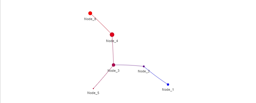

OPTION #2 (all process integrate in the same function):

It creates the GSSTDA object with full data set, internally pre-process using the DGSA technique, and the mapper information.

GSSTDA_obj <- GSSTDA(full_data = full_data, survival_time = survival_time, 
                     survival_event = survival_event, case_tag = case_tag, 
                     gen_select_type = gen_select_type, 
                     percent_gen_select = percent_gen_select, 
                     num_intervals = num_intervals, 
                     percent_overlap = percent_overlap, 
                     distance_type = distance_type, 
                     clustering_type = clustering_type, 
                     linkage_type = linkage_type)

Obtain information from the DGSA block created in the previous step.

This function returns the 100 genes with the highest variability within the dataset and builds a heat map with them.

DGSA_information <- results_DGSA(GSSTDA_obj[["matrix_disease_component"]], case_tag)
print(DGSA_information)

Obtain information from the mapper object created in the G-SS-TDA process.

print(GSSTDA_obj[["mapper_obj"]])

Plot the mapper graph.

plot_mapper(GSSTDA_obj[["mapper_obj"]])