
In a quality statistical data analysis the initial step has to be exploratory. Exploratory data analysis begins with the univariate exploratory analyis - examining the variable one at a time. Next comes bivariate analysis followed by multivariate analyis. SmartEDA package helps in getting the complete exploratory data analysis just by running the function instead of writing lengthy r code.
The SmartEDA R package has four unique functionalities as
SmartEDA package with other similar packages available in CRAN for exploratory data analysis viz. dlookr, DataExplorer, Hmisc, exploreR, RtutoR and summarytools. The metric for evaluation is the availability of various desired features for performing an Exploratory data analysis
An article describing SmartEDA package for exploratory data analysis approach has been published in arxiv and Journal of Open Source Software JOSS. Please cite the paper if you use SmartEDA in your work!
The package can be installed directly from CRAN.
install.packages("SmartEDA")You can install the latest development verion of the SmartEDA from github with:
install.packages("devtools")
devtools::install_github("daya6489/SmartEDA",ref = "develop")In this vignette, we will be using a simulated data set containing sales of child car seats at 400 different stores.
Data Source ISLR package.
Install the package “ISLR” to get the example data set.
    install.packages("ISLR")
    library("ISLR")
    install.packages("SmartEDA")
    library("SmartEDA")
    ## Load sample dataset from ISLR pacakge
Carseats= ISLR::CarseatsUnderstanding the dimensions of the data set, variable names, overall missing summary and data types of each variables
## overview of the data;
    ExpData(data=Carseats,type=1)
## structure of the data
ExpData(data=Carseats,type=2)To summarise the numeric variables, you can use following r codes from this pacakge
## Summary statistics by – overall
    ExpNumStat(Carseats,by="A",gp=NULL,Qnt=seq(0,1,0.1),MesofShape=2,Outlier=TRUE,round=2)
## Summary statistics by – overall with correlation
    ExpNumStat(Carseats,by="A",gp="Price",Qnt=seq(0,1,0.1),MesofShape=1,Outlier=TRUE,round=2)
## Summary statistics by – category
ExpNumStat(Carseats,by="GA",gp="Urban",Qnt=seq(0,1,0.1),MesofShape=2,Outlier=TRUE,round=2)ExpNumStat(mtcars,by="A",round=2, weight = "wt")## Generate Boxplot by category
ExpNumViz(mtcars,target="gear",type=2,nlim=25,fname = file.path(tempdir(),"Mtcars2"),Page = c(2,2))
## Generate Density plot
ExpNumViz(mtcars,target=NULL,type=3,nlim=25,fname = file.path(tempdir(),"Mtcars3"),Page = c(2,2))
## Generate Scatter plot
ExpNumViz(mtcars,target="carb",type=3,nlim=25,fname = file.path(tempdir(),"Mtcars4"),Page = c(2,2))## Frequency or custom tables for categorical variables
ExpCTable(Carseats,Target=NULL,margin=1,clim=10,nlim=5,round=2,bin=NULL,per=T)
ExpCTable(Carseats,Target="Price",margin=1,clim=10,nlim=NULL,round=2,bin=4,per=F)
ExpCTable(Carseats,Target="Urban",margin=1,clim=10,nlim=NULL,round=2,bin=NULL,per=F)
## Summary statistics of categorical variables
ExpCatStat(Carseats,Target="Urban",result = "Stat",clim=10,nlim=5,Pclass="Yes")
## Inforamtion value and Odds value
ExpCatStat(Carseats,Target="Urban",result = "IV",clim=10,nlim=5,Pclass="Yes")ExpCTable(mtcars, margin = 1, clim = 10, nlim = 3, bin = NULL, per = FALSE, weight = "wt"")## column chart
ExpCatViz(Carseats,target="Urban",fname=NULL,clim=10,col=NULL,margin=2,Page = c(2,1),sample=2)
## Stacked bar graph
ExpCatViz(Carseats,target="Urban",fname=NULL,clim=10,col=NULL,margin=2,Page = c(2,1),sample=2)
## Variable importance graph using information values
ExpCatStat(Carseats,Target="Urban",result="Stat",Pclass="Yes",plot=TURE,top=20,Round=2) ExpCatStat(Carseats,Target="Urban",result = "Stat",clim=10,nlim=5,bins=10,Pclass="Yes",plot=TRUE,top=10,Round=2)Create a exploratory data analysis report in HTML format
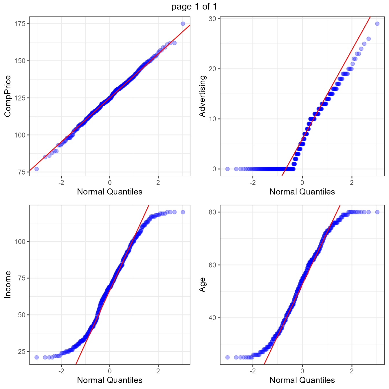
ExpReport(Carseats,Target="Urban",label=NULL,op_file="test.html",op_dir=getwd(),sc=2,sn=2,Rc="Yes") ExpOutQQ(CData,nlim=10,fname=NULL,Page=c(2,2),sample=4)
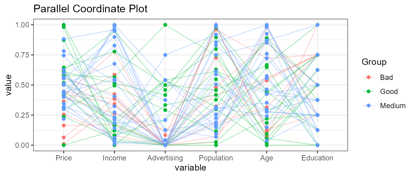
## Defualt ExpParcoord funciton
    ExpParcoord(CData,Group=NULL,Stsize=NULL,Nvar=c("Price","Income","Advertising","Population","Age","Education"))
## With Stratified rows and selected columns only
  ExpParcoord(CData,Group="ShelveLoc",Stsize=c(10,15,20),Nvar=c("Price","Income"),Cvar=c("Urban","US"))
## Without stratification
  ExpParcoord(CData,Group="ShelveLoc",Nvar=c("Price","Income"),Cvar=c("Urban","US"),scale=NULL)
## Scale change
  ExpParcoord(CData,Group="US",Nvar=c("Price","Income"),Cvar=c("ShelveLoc"),scale="std")
## Selected numeric variables
  ExpParcoord(CData,Group="ShelveLoc",Stsize=c(10,15,20),Nvar=c("Price","Income","Advertising","Population","Age","Education"))
## Selected categorical variables
  ExpParcoord(CData,Group="US",Stsize=c(15,50),Cvar=c("ShelveLoc","Urban"))
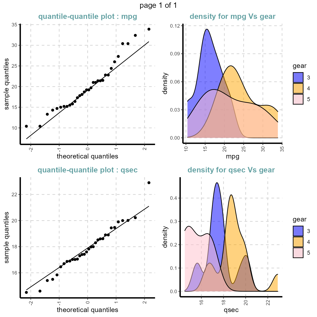
To plot graph from same variable when Target=NULL vs. when Target = categorical variable (binary or multi-class variable)
target = "gear"
categorical_features <- c("vs", "am", "carb")
numeircal_features <- c("mpg", "cyl", "disp", "hp", "drat", "wt", "qsec")

num_1 <- ExpTwoPlots(mtcars,
                     plot_type = "numeric",
                     iv_variables = numeircal_features,
                     target = "gear",
                     lp_arg_list = list(alpha=0.5, color = "red", fill= "white", binwidth=1),
                     lp_geom_type = 'histogram',
                     rp_arg_list = list(alpha=0.5, fill = c("red", "orange", "pink"),  binwidth=1),
                     rp_geom_type = 'histogram',
                     fname = "dub2.pdf",
                     page = c(2,1),
                     theme = "Default")
In statistics, an outlier is a data point that differs significantly from other observations. An outlier may be due to variability in the measurement or it may indicate experimental error; the latter are sometimes excluded from the data set.An outlier can cause serious problems in statistical analyses.
Identifying outliers: There are several methods we can use to identify outliers. In ExpOutliers used two methods (1) Boxplot and (2) Standard Deviation

##Identifying outliers mehtod - Boxplot
ExpOutliers(Carseats, varlist = c("Sales","CompPrice","Income"), method = "boxplot",  capping = c(0.1, 0.9))

##Identifying outliers mehtod - 3 Standard Deviation
ExpOutliers(Carseats, varlist = c("Sales","CompPrice","Income"), method = "3xStDev",  capping = c(0.1, 0.9))

##Identifying outliers mehtod - 2 Standard Deviation
ExpOutliers(Carseats, varlist = c("Sales","CompPrice","Income"), method = "2xStDev",  capping = c(0.1, 0.9))


##Create outlier flag (1,0) if there are any outliers
ExpOutliers(Carseats, varlist = c("Sales","CompPrice","Income"), method = "3xStDev",  capping = c(0.1, 0.9), outflag = TRUE)

##Impute outlier value by mean or median valie
ExpOutliers(Carseats, varlist = c("Sales","CompPrice","Income"), method = "3xStDev", treatment = "mean", capping = c(0.1, 0.9), outflag = TRUE)Descriptive summary on all input variables for each level/combination of group variable. Also while running the analysis we can filter row/cases of the data.
    ExpCustomStat(Carseats,Cvar=c("US","Urban","ShelveLoc"),gpby=FALSE)
    ExpCustomStat(Carseats,Cvar=c("US","Urban"),gpby=TRUE,filt=NULL)
    ExpCustomStat(Carseats,Cvar=c("US","Urban","ShelveLoc"),gpby=TRUE,filt=NULL)
    ExpCustomStat(Carseats,Cvar=c("US","Urban"),gpby=TRUE,filt="Population>150")
    ExpCustomStat(Carseats,Cvar=c("US","ShelveLoc"),gpby=TRUE,filt="Urban=='Yes' & Population>150")
    ExpCustomStat(Carseats,Nvar=c("Population","Sales","CompPrice","Income"),stat = c('Count','mean','sum','var','min','max'))
    ExpCustomStat(Carseats,Nvar=c("Population","Sales","CompPrice","Income"),stat = c('min','p0.25','median','p0.75','max'))
    ExpCustomStat(Carseats,Nvar=c("Population","Sales","CompPrice","Income"),stat = c('Count','mean','sum','var'),filt="Urban=='Yes'")
    ExpCustomStat(Carseats,Nvar=c("Population","Sales","CompPrice","Income"),stat = c('Count','mean','sum'),filt="Urban=='Yes' & Population>150")
    ExpCustomStat(data_sam,Nvar=c("Population","Sales","CompPrice","Income"),stat = c('Count','mean','sum','min'),filt="All %ni% c(999,-9)")
    ExpCustomStat(Carseats,Nvar=c("Population","Sales","CompPrice","Education","Income"),stat = c('Count','mean','sum','var','sd','IQR','median'),filt=c("ShelveLoc=='Good'^Urban=='Yes'^Price>=150^ ^US=='Yes'"))
    ExpCustomStat(Carseats,Cvar = c("Urban","ShelveLoc"), Nvar=c("Population","Sales"), stat = c('Count','Prop','mean','min','P0.25','median','p0.75','max'),gpby=FALSE)
    ExpCustomStat(Carseats,Cvar = c("Urban","US","ShelveLoc"), Nvar=c("CompPrice","Income"), stat = c('Count','Prop','mean','sum','PS','min','max','IQR','sd'), gpby = TRUE)
    ExpCustomStat(Carseats,Cvar = c("Urban","US","ShelveLoc"), Nvar=c("CompPrice","Income"), stat = c('Count','Prop','mean','sum','PS','P0.25','median','p0.75'), gpby = TRUE,filt="Urban=='Yes'")
    ExpCustomStat(data_sam,Cvar = c("Urban","US","ShelveLoc"), Nvar=c("Sales","CompPrice","Income"), stat = c('Count','Prop','mean','sum','PS'), gpby = TRUE,filt="All %ni% c(888,999)")
ExpCustomStat(Carseats,Cvar = c("Urban","US"), Nvar=c("Population","Sales","CompPrice"), stat = c('Count','Prop','mean','sum','var','min','max'), filt=c("ShelveLoc=='Good'^Urban=='Yes'^Price>=150"))See article wiki page.