The package VisitorCounts offers tools to estimate and forecast the number of visitors or its percent changes to National Parks. Our method works by employing singular spectrum analysis (SSA) to decompose park-level photo-user-days (PUD) into estimated trend and seasonal components. Here, PUD is the number of unique users per day that shared an image from within a target location (such as the number of unique users per day that shared geo-tagged Flickr images of the Yosemite National Park). Following appropriate adjustments, these components can be used as estimates or forecasts for the trend and seasonality components of \(\Delta\) log\((N_{i,t})\) (where \(N_{i,t} > 0\) denote the actual visitor counts in month \(t\) at park \(i\)). Therefore, by using the VisitorCounts package, one can find the estimated or forecasted percent change in a park’s visitor counts by only using social media data for that park. Our model is unique in that, whereas other models partially or fully utilize on-site visitor counts, ours can achieve competitive performances on visitation forecasts only with the use of social media data. In addition, visitation forecasts can be improved by combining PUD with partial or full on-site visitor counts.
An example of using the VisitorCounts package is forecast- ing the number of visitors to a national park for a specific month. Lets estimate the number of visitors to the Yosemite National Park for the month of August in 2022 using a model that relies on social media data and previous on-site counts.
First load the VisitorCounts package:
library("VisitorCounts")
#> Warning: package 'VisitorCounts' was built under R version 4.2.3
#> Registered S3 method overwritten by 'quantmod':
#>   method            from
#>   as.zoo.data.frame zoo
With VisitorCounts loaded, you will need to load the appropriate data sets:
data("park_visitation")The park_visitation data set will be used to get the Flickr PUD data for the Yosemite National Park. The flickr_userdays data set will be used as a proxy for the popularity of Flickr when creating a visitation_model object.
Let us then extract the Yosemite dataset and put it into a time series with these two commands:
yosemite_pud <- park_visitation[park_visitation$park == "YOSE",]$pud #PUD data
yosemite_nps <- park_visitation[park_visitation$park == "YOSE",]$nps #On site recorded visitation
Before we create a Visitation_Model object, we should log-transform both the flickr_userdays and yosemite_pud for the best results.
log_yosemite_pud <- log(yosemite_pud)

log_yosemite_nps <- log(yosemite_nps)
Now we can create our visitation_model that we will be doing predictions with:
yose_visitation_model <- visitation_model(ref_series = log_yosemite_nps, onsite_usage = log_yosemite_pud, omit_trend = TRUE, parameter_estimates = "joint", is_output_logged = FALSE, is_input_logged = TRUE)
#> All the forecasts will be made in the log scale.
With this model, we will now be able to create our forecasts:
yosemite_visitation_forecasts <- predict(yose_visitation_model, n_ahead = 60)$forecast[1:60] In this context n_ahead represents the number of months we will be forecasting.I put the value as 60 because since our time series has data up until the end of 2017 and I want to forecast for a month in 2022 I will need to create forecasts for all the months through 2018 up until that month in 2022. Alternatively, if n_ahead had been set to 12 I would only generate forecasts through the year of 2018.
Now we can plot these forecasts and look at the graph with the commands:
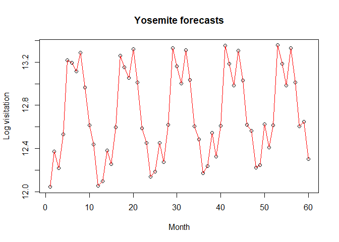
plot(yosemite_visitation_forecasts, main="Yosemite forecasts", type="l",xlab="Month", ylab="Log visitation")
points(yosemite_visitation_forecasts)
lines(yosemite_visitation_forecasts, col="red")
The graph is labeled as the number of months after the training data predicted on the x-axis and the y axis is log base e of the visitation to the park. Since our training data ends at 2017, one can read the graph by selecting the numbered month after 2017 that they are interested in. In our case we are looking for the number of visitors for August 2022, which would be the 56th month after the end of 2017. By looking at our graph we can see that the 56th month is about 13. Moreover to get an actual estimate for visitation we calculate \(e^{13} = 442,413\), which would be the expected number of visitors based on our model.
You can install the current version of VisitorCounts with:
install.packages("VisitorCounts")You can view an in-depth explanation of the main components for this package through the included vignette.