Our package uses state-of-the-art state-space models to facilitate the modeling and forecasting of financial intraday signals. It currently offers a univariate model for intraday trading volume, with new features on intraday volatility and multivariate models in development. It is a valuable tool for anyone interested in exploring intraday, algorithmic, and high-frequency trading.
The package can be installed from GitHub:
# install development version from GitHub
devtools::install_github("convexfi/intradayModel")
Please cite intradayModel in publications:
citation("intradayModel")To get started, we load our package and sample data: the 15-minute intraday trading volume of AAPL from 2019-01-02 to 2019-06-28, covering 124 trading days. We use the first 104 trading days for fitting, and the last 20 days for evaluation of forecasting performance.
library(intradayModel)
data(volume_aapl)
volume_aapl[1:5, 1:5] # print the head of data
#>          2019-01-02 2019-01-03 2019-01-04 2019-01-07 2019-01-08
#> 09:30 AM   10142172    3434769   20852127   15463747   14719388
#> 09:45 AM    5691840   19751251   13374784    9962816    9515796
#> 10:00 AM    6240374   14743180   11478596    7453044    6145623
#> 10:15 AM    5273488   14841012   16024512    7270399    6031988
#> 10:30 AM    4587159   18041115    8686059    7130980    5479852

volume_aapl_training <- volume_aapl[, 1:104]
volume_aapl_testing <- volume_aapl[, 105:124]
Next, we fit a univariate state-space model using
fit_volume() function.
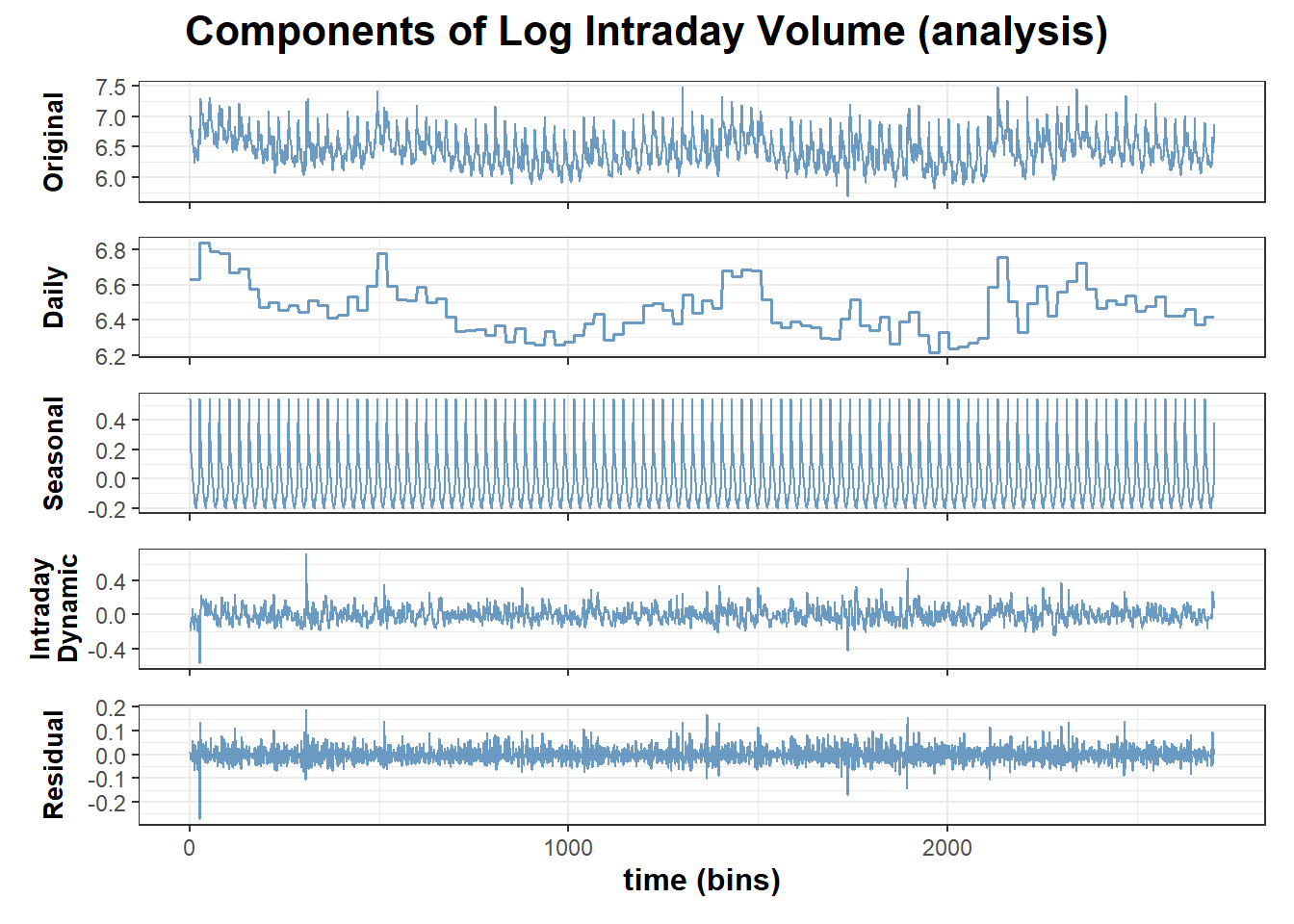
model_fit <- fit_volume(volume_aapl_training)Once the model is fitted, we can analyze the hidden components of any
intraday volume based on all its observations. By calling
decompose_volume() function with
purpose = "analysis", we obtain the smoothed daily,
seasonal, and intraday dynamic components. It involves incorporating
both past and future observations to refine the state estimates.
analysis_result <- decompose_volume(purpose = "analysis", model_fit, volume_aapl_training)

# visualization
plots <- generate_plots(analysis_result)
plots$log_components
To see how well our model performs on new data, we call
forecast_volume() function to do one-bin-ahead forecast on
the testing set.
forecast_result <- forecast_volume(model_fit, volume_aapl_testing)

# visualization
plots <- generate_plots(forecast_result)
plots$original_and_forecast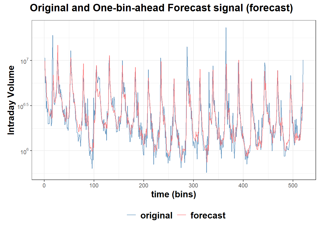
We welcome all sorts of contributions. Please feel free to open an issue to report a bug or discuss a feature request.
If you make use of this software please consider citing:
Package: GitHub
Vignette: GitHub-vignette.